WebMO and Jupyter Notebooks

WebMO Enterprise and Jupyter Notebooks make a powerful combination for the analysis and visualization of computational chemistry results. Using the REST interface (WebMO Enterprise), you can retrieve results from existing WebMO calculations and then interactively analyze those results (via Python) right inside a Jupyter notebook.

Getting Started

Basic information about configuring WebMO to work with Jupyter notebooks can be found in the WebMO documentation. You can use a Jupyter Notebook that has been installed right on your own desktop / laptop computer (most common) or via a centralized installation via services such as Jupyter Hub or MyBinder. Alternative, any standard Python installation can also be used, although some of the interactive visualization features of Jupyter cannot be utilized.

Accessing WebMO Jobs Using Jupyter

Results from previously run WebMO jobs can be accessed and then analyzed in numerous ways using standard Python commands and libraries. Several useful example Python templates are provided with the standard WebMO distribution (e.g. geometry optimization convergence, plotting orbital energy level diagrams, thermochemistry...). These examples also serve as a simple "templates" for limitless instructor or student-generated possibilities.

In each case, the basic workflow is the same:

1. Authenticate with the REST interface using a WebMO username/password
2. Retrieve the results for the desired WebMO calculation
3. Analyze/plot the results, as desired, using standard Python/Juypter commands

The standard WebMO installation comes with a number of "template" example Python scripts that implement the above workflow:

• Printing a list of calculated quantities
• Plotting coordinate scan energies
• Plotting the convergence of a geometry optimization
• Generating a molecular orbital diagram
• Calculating basic thermochemistry

This basic workflow is illustrated in the annotated example below, which shows how to generate a standard orbital diagram by plotting the MO energy levels of a molecule.

Annotated Example

This first block of code simply import the various libraries that we require for accessing the REST API and for doing some basic visualization (using MatPlotLib). In this case, we will be accessing the MatPlotLib functionality via the "plt" variable:

import requests
from getpass import getpass
import json

import math
%matplotlib notebook
import matplotlib.pyplot as plt

Next, we define the location of the target WebMO installation and the username of the associated WebMO user whose job we wish to access:

baseURL="https://webmo.myserver.edu/~webmo/cgi-bin/webmo/rest.cgi"
username="smith"
jobNumber=962

Finally, we complete the authentication process by posting the username / password combination (the latter obtained form the keyboard, in this case) to the REST service, receiving a valid REST token in response; the latter is used to authenticate all subsequent request.

print("Enter WebMO password:")
password=getpass()
try:
    #obtain a REST token
    login={'username' : username, 'password' : password} #WebMO login information, used to retrieve a REST access token
    r = requests.post(baseURL + "/sessions", data=login)
    r.raise_for_status() #raise an exception if there is a problem with the request
    auth=r.json() #include both 'username' and 'token' parameters needed to authenticate further REST requests

Next, we can request the results for the WebMO job of interest. The results are returned in a JSON data structure that is decoded into a standard Python dictionary named "results". We also read out a few interesting values from that dictionary (final geometry, list of atomic symbols, and a dictionary of calculated properties):

    #obtain results from the specified job number
    r = requests.get(baseURL + "/jobs/%d/results" % jobNumber, params=auth)
    r.raise_for_status() #raise an exception if there is a problem with the request
    results=r.json()
    
    #read out the optimized geometry and properties
    geometry=results["geometry"]
    symbols=results["symbols"]
    properties=results["properties"]

Here is where the "meat" of this particular example occurs. We first read the energies and occupancies of the molecular orbitals from the "properties" dictionary, loop over the orbital energies, and then plot the energy levels using MatPlotLib:

    #sanity check: verify this was some sort of optimization
    if "orbitals" not in properties:
        raise ValueError("No molecular orbital data found: not a molecular orbital calculation?")
    
    #read out the orbital information; plotting restricted (or alpha-spin) MOs by default
    alpha_or_restricted=0
    beta=1
    energies=properties["orbitals"]["energies"][alpha_or_restricted]
    occupancies=properties["orbitals"]["occupancy"][alpha_or_restricted]
    
    #now draw the MO diagram
    fig, ax1 = plt.subplots()
    
    plt.xlim([-5,5])
    ax1.set_ylabel('Energy')
    ax1.get_xaxis().set_visible(False)
        
    for i in range(0,len(energies)):
        
        #search forward and backward to find other orbitals of the same energy
        backward_degeneracy=0
        forward_degeneracy=0
        while i-backward_degeneracy-1 >= 0 and energies[i-backward_degeneracy-1] == energies[i]:
            backward_degeneracy+=1
        while i+forward_degeneracy+1 < len(energies) and energies[i+forward_degeneracy+1] == energies[i]:
            forward_degeneracy+=1
        degeneracy = backward_degeneracy + forward_degeneracy + 1
        #calculate the proper position of the orbital line based on the degeneracy
        offset = (degeneracy - 1) / 2 - backward_degeneracy 
        
        #stylize, using black for occupied and red for unoccupied MOs
        if occupancies[i] > 0:
            style="k-"
        else:
            style="r-"
            
        ax1.plot([-0.4 - offset,0.4 - offset], [energies[i],energies[i]], style, lw=1)

After competing the calculations, it is good practice to delete the REST session to prevent unauthorized access:

    #End the REST session
    r = requests.delete(baseURL + "/sessions", params=auth)
    r.raise_for_status() #raise an exception if there is a problem with the request

This last bit of code is just provides some exception (error) handling in case anything goes wrong with any of the prior requests:

#
#Catch any HTTP / REST exceptions and log the underlying cause
#
except requests.exceptions.HTTPError:
    if (r.ok):
        print("Error during REST request: %s" % r.json()["error"])
    else:
        print("HTTP error: %s" % r.reason)

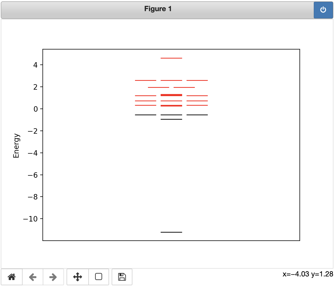
Running the above code then generates a conventional MO diagram (for CH₄, in this case), where occupied orbitals are shown in black and unoccupied (virtual) orbitals in red: